Bayesian Mixed Graphical Model

Introduction

In this example, we illustrate the use of the BMGM package to infer conditional independence relationships among mixed-type variables using data from the NHANES study. Our model can handle continuous, binary, and count variables, and allows for missing values using a data augmentation strategy.

Load required packages

library(BMGM)
library(NHANES)
#> Warning: package 'NHANES' was built under R version 4.4.3
library(dplyr)
#> 
#> Attaching package: 'dplyr'
#> The following objects are masked from 'package:stats':
#> 
#>     filter, lag
#> The following objects are masked from 'package:base':
#> 
#>     intersect, setdiff, setequal, union
library(qgraph)

Data Preparation

We select six variables from the NHANES dataset that are common in health studies:

Age: Continuous variable (in years)
Gender: Categorical variable (1 = male, 2 = female)
SleepHrsNight: Discrete variable (typical sleep per night)
BPSysAve: Continuous variable (average systolic blood pressure)
BMI: Continuous variable (Body Mass Index)
Diabetes: Categorical variable (1 = no, 2 = yes)

We filter rows with at most 2 missing values to allow for imputation during inference.

set.seed(123)

data <- NHANES %>%
  select(Age, Gender, SleepHrsNight, BPSysAve, BMI, Diabetes) %>%
  filter(rowSums(is.na(.)) <= 2, Age > 18) %>%
  mutate(
    Gender = ifelse(Gender == "female", 2,
             ifelse(Gender == "male", 1, NA)),
    Diabetes = ifelse(Diabetes == "Yes", 2,
               ifelse(Diabetes == "No", 1, NA))
  ) %>%
  slice_sample(n = 300) %>%
  as.matrix()

Define the variable types:

type <- c("c", "m", "d", "c", "c", "m")
var_names <- c("Age", "Gender", "Sleep", "BP_sys", "BMI", "Diabetes")

Fit the Model

We run the Bayesian mixed graphical model with default priors and 2,000 burn-in and sampling iterations. You can increase this number for more stable results.

fit <- bmgm(data, type = type, nburn = 2000, nsample = 2000, seed = 123)

Visualize the Inferred Graph

We use the qgraph package to visualize the graph. Edge width corresponds to the strength of the relationship, and edge color indicates direction:

Green = positive interaction
Red = negative interaction

qgraph(
  fit$adj_Beta,
  labels = var_names,
  edge.color = ifelse(fit$adj_Beta > 0, "darkgreen", "firebrick"),
  edge.width = abs(fit$adj_Beta)*2,
  layout = "spring",
  vsize = 6
)

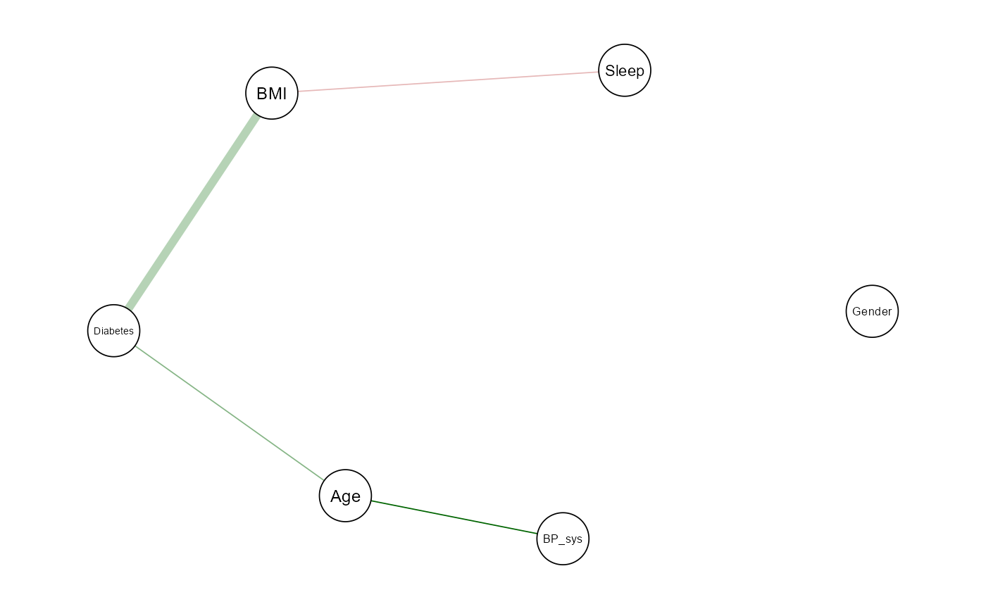
Interpretation

Age ↔︎ BP_sys (Systolic Blood Pressure) A positive conditional relationship (0.71) reflects the expected pattern: as age increases, systolic blood pressure tends to increase, consistent with physiological changes over time.
Age ↔︎ Diabetes A positive edge (0.34) suggests that age is positively associated with diabetes, even after adjusting for BMI and other variables.
BMI ↔︎ Diabetes A positive edge (0.20) indicates that BMI is conditionally associated with the presence of diabetes. This supports the well-established clinical link between higher body mass index and type 2 diabetes.
Sleep ↔︎ BMI A weak negative edge (-0.23) implies a minor inverse relationship between BMI and sleep duration. While small, this may hint at patterns where higher BMI is associated with slightly lower average sleep time.
Gender Gender remains conditionally independent of the rest of the variables, as it is disconnected in the estimated graph.

This model accounts for missing data via MCMC-based imputation and uses a spike-and-slab prior to identify sparse graphs, allowing meaningful discovery of variable interactions. Gender and Diabetes are treated as categorical variables (type "m") rather than count data, reflecting their true nature as binary categories.

Summary

This vignette demonstrates how to use the BMGM package to analyze real-world health data involving mixed variable types. The method flexibly models continuous, binary, and count variables, and is robust to small amounts of missing data. Future work may extend this example to include zero-inflated variables or longitudinal data.