require(rstanarm)
require(rstantools)
require(bayesplot)Predicting Euro & Copa America - 2024
A statistical model to analyze the results of the Euro Cup and the Copa America 2024.
In this project, I will propose a model for predicting the Euro & Copa America - 2024 scores based on the model presented in (Florez, Guindani, and Vannucci 2024).
Packages
I will use a Bayesian model, so we need the following libraries
As well as
require(readr)
require(dplyr)
require(lubridate)
require(ggplot2)
require(ggrepel)
require(latex2exp)
Data
The data is contained in this repository https://github.com/martj42/international_results.
urlfile = "https://raw.githubusercontent.com/martj42/international_results/master/results.csv"We load the data
data <- read_csv(url(urlfile), show_col_types = FALSE)The proposed model is based on the teams’ strengths attacking and defending. To train the model, we used the scores of games played since season 2023-2024.
euro_2024 = c('Albania','Austria','Belgium','Croatia','Czech Republic','Denmark','England','France','Georgia','Germany','Hungary','Italy','Netherlands','Poland','Portugal','Romania','Scotland','Serbia','Slovakia','Slovenia','Spain','Switzerland','Turkey','Ukraine')

america_2024 = sort(c('Argentina', 'Chile', 'Peru', 'Canada', 'Mexico', 'Ecuador', 'Venezuela', 'Jamaica', 'United States', 'Uruguay', 'Panama', 'Bolivia', 'Brazil', 'Colombia', 'Paraguay', 'Costa Rica'))

scores <- data %>%
  filter(home_team %in% euro_2024 & away_team %in% euro_2024) %>%
  filter(date > "2023-06-01") %>%
  mutate(id = row_number(), cup = "Euro") %>%
  bind_rows(data %>%
  filter(home_team %in% america_2024 & away_team %in% america_2024) %>%
  filter(date > "2023-06-01") %>%
  mutate(id = row_number(), cup = "America")
  )
For example, we consider the following games played by Portugal.
scores %>%
  filter(home_team == "Portugal" | away_team == "Portugal")
# A tibble: 21 × 11
date home_team away_team home_score away_score tournament city country
<date> <chr> <chr> <dbl> <dbl> <chr> <chr> <chr>
1 2023-09-08 Slovakia Portugal 0 1 UEFA Euro… Brat… Slovak…
2 2023-10-13 Portugal Slovakia 3 2 UEFA Euro… Porto Portug…
3 2024-03-26 Slovenia Portugal 2 0 Friendly Ljub… Sloven…
4 2024-06-08 Portugal Croatia 1 2 Friendly Oeir… Portug…
5 2024-06-18 Portugal Czech Re… 2 1 UEFA Euro Leip… Germany
6 2024-06-22 Turkey Portugal 0 3 UEFA Euro Dort… Germany
7 2024-06-26 Georgia Portugal 2 0 UEFA Euro Gels… Germany
8 2024-07-01 Portugal Slovenia 0 0 UEFA Euro Fran… Germany
9 2024-07-05 Portugal France 0 0 UEFA Euro Hamb… Germany
10 2024-09-05 Portugal Croatia 2 1 UEFA Nati… Lisb… Portug…
# ℹ 11 more rows
# ℹ 3 more variables: neutral <lgl>, id <int>, cup <chr>and the following games played by Colombia
scores %>%
  filter(home_team == "Colombia" | away_team == "Colombia")
# A tibble: 29 × 11
date home_team away_team home_score away_score tournament city country
<date> <chr> <chr> <dbl> <dbl> <chr> <chr> <chr>
1 2023-09-07 Colombia Venezuela 1 0 FIFA Worl… Barr… Colomb…
2 2023-09-12 Chile Colombia 0 0 FIFA Worl… Sant… Chile
3 2023-10-12 Colombia Uruguay 2 2 FIFA Worl… Barr… Colomb…
4 2023-10-17 Ecuador Colombia 0 0 FIFA Worl… Quito Ecuador
5 2023-11-16 Colombia Brazil 2 1 FIFA Worl… Barr… Colomb…
6 2023-11-21 Paraguay Colombia 0 1 FIFA Worl… Asun… Paragu…
7 2023-12-16 Mexico Colombia 2 3 Friendly Los … United…
8 2024-06-08 United S… Colombia 1 5 Friendly Land… United…
9 2024-06-15 Colombia Bolivia 3 0 Friendly Denv… United…
10 2024-06-24 Colombia Paraguay 2 1 Copa Amér… Hous… United…
# ℹ 19 more rows
# ℹ 3 more variables: neutral <lgl>, id <int>, cup <chr>Filtering data
home_scores <- scores %>%
  select(id, score = home_score, team = home_team, adversary = away_team, date = date, cup) %>%
  mutate(condition = ifelse(scores$neutral, "neutral", "home"))

away_scores <- scores %>%
  select(id, score = away_score, team = away_team, adversary = home_team, date = date, cup) %>%
  mutate(condition = ifelse(scores$neutral, "neutral", "away"))

total_scores <- union_all(home_scores, away_scores)
We also consider the ranking FIFA of the teams as covariate. For every game, select the up-to-date ranking
path0 <- "https://raw.githubusercontent.com/Dato-Futbol/fifa-ranking/master/ranking_fifa_historical.csv"
rank <- read_csv(url(path0), show_col_types = FALSE)

rank <- rank %>%
  select(team, total_points, date) %>%
  group_by(date) %>%
  mutate(ranking = rank(-total_points))
Merging the data will be
scores_rank <- total_scores %>%
  left_join(rank, by = join_by(adversary == team), relationship = "many-to-many") %>%
  filter(date.x >= date.y) %>%
  mutate(diff_date = date.x - date.y) %>%
  group_by(id, team) %>%
  slice_min(diff_date) %>%
  select(id, score, team, adversary, condition, date_game = date.x, ranking_adv = ranking, date_rank = date.y, cup)
We are separating the data for both Euro and Copa America. For both cases, we will use as test data the games played after the quarter-finals. i.e, we will finish predicting the results of the semi-finals and the finals.
date_euro = "2024-07-09"
date_ca = "2024-07-09"

train_euro <- scores_rank %>%
  filter(date_game < date_euro, cup == "Euro")

train_america <- scores_rank %>%
  filter(date_game < date_ca, cup == "America")

test_euro <- scores_rank %>%
  filter(date_game >= date_euro, cup == "Euro")

test_america <- scores_rank %>%
  filter(date_game >= date_ca, cup == "America")
Fitting the model
To fit the model I would consider the scores are distributed as Poisson for simplicity, one better option is the Conway-Maxwell-Poisson as shown in (Florez, Guindani, and Vannucci 2024). However, we will use a simple model for computational reasons as we constantly update the model.
model_euro <- stan_glm(score ~ 1 + team + adversary + condition + ranking_adv, data = train_euro, family = poisson, iter = 5000, contrasts = list(team = "contr.sum", adversary = "contr.sum"))model_america <- stan_glm(score ~ 1 + team + adversary + condition + ranking_adv, data = train_america, family = poisson, iter = 5000, contrasts = list(team = "contr.sum", adversary = "contr.sum"))Estimation
Euro
strength_att <- model_euro$coefficients[2:24]
strength_att <- c(strength_att, 0 - sum(strength_att))

strength_def <- model_euro$coefficients[25:47]
strength_def <- c(strength_def, 0 - sum(strength_def))

coeffs <- data.frame(team = euro_2024, strength_att, strength_def, row.names = c())
Now, we can plot the estimated strengths in the following way:
ggplot(coeffs, aes(x = strength_att, y = -strength_def)) +
  geom_hline(yintercept = 0, linetype = "dashed", color = "grey50") +
  geom_vline(xintercept = 0, linetype = "dashed", color = "grey50") +
  geom_point() +
  geom_label_repel(aes(label = team),
                            box.padding = 0.25,
                            point.padding = 0.5,
                            segment.color = "grey50") +
  xlab(expression("Better Attack" %->% "")) +
  ylab(expression("Better Defense" %->% "")) +
  ggtitle("Strengths of every team") +
  theme_classic() +
  theme(plot.title = element_text(hjust = 0.5))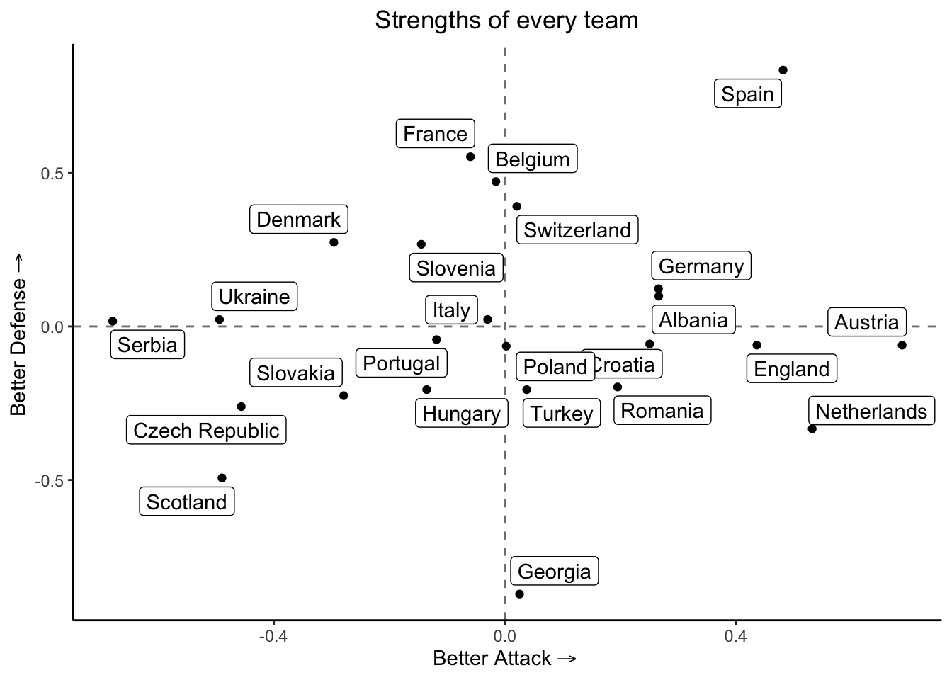
This graph provides an intuition into the strengths and abilities of every team. Teams located in the origin have an overall performance, and below the axis are worse than the averages’ team.
Copa America
Similarly for Copa america
n <- length(america_2024)
strength_att <- model_america$coefficients[2:n]
strength_att <- c(strength_att, 0 - sum(strength_att))

strength_def <- model_america$coefficients[(n+1):(2*n-1)]
strength_def <- c(strength_def, 0 - sum(strength_def))

coeffs <- data.frame(team = america_2024, strength_att, strength_def, row.names = c())
Now, we can plot the estimated strengths in the following way:
ggplot(coeffs, aes(x = strength_att, y = -strength_def)) +
  geom_hline(yintercept = 0, linetype = "dashed", color = "grey50") +
  geom_vline(xintercept = 0, linetype = "dashed", color = "grey50") +
  geom_point() +
  geom_label_repel(aes(label = team),
                            box.padding = 0.25,
                            point.padding = 0.5,
                            segment.color = "grey50") +
  xlab(expression("Better Attack" %->% "")) +
  ylab(expression("Better Defense" %->% "")) +
  ggtitle("Strengths of every team") +
  theme_classic() +
  theme(plot.title = element_text(hjust = 0.5))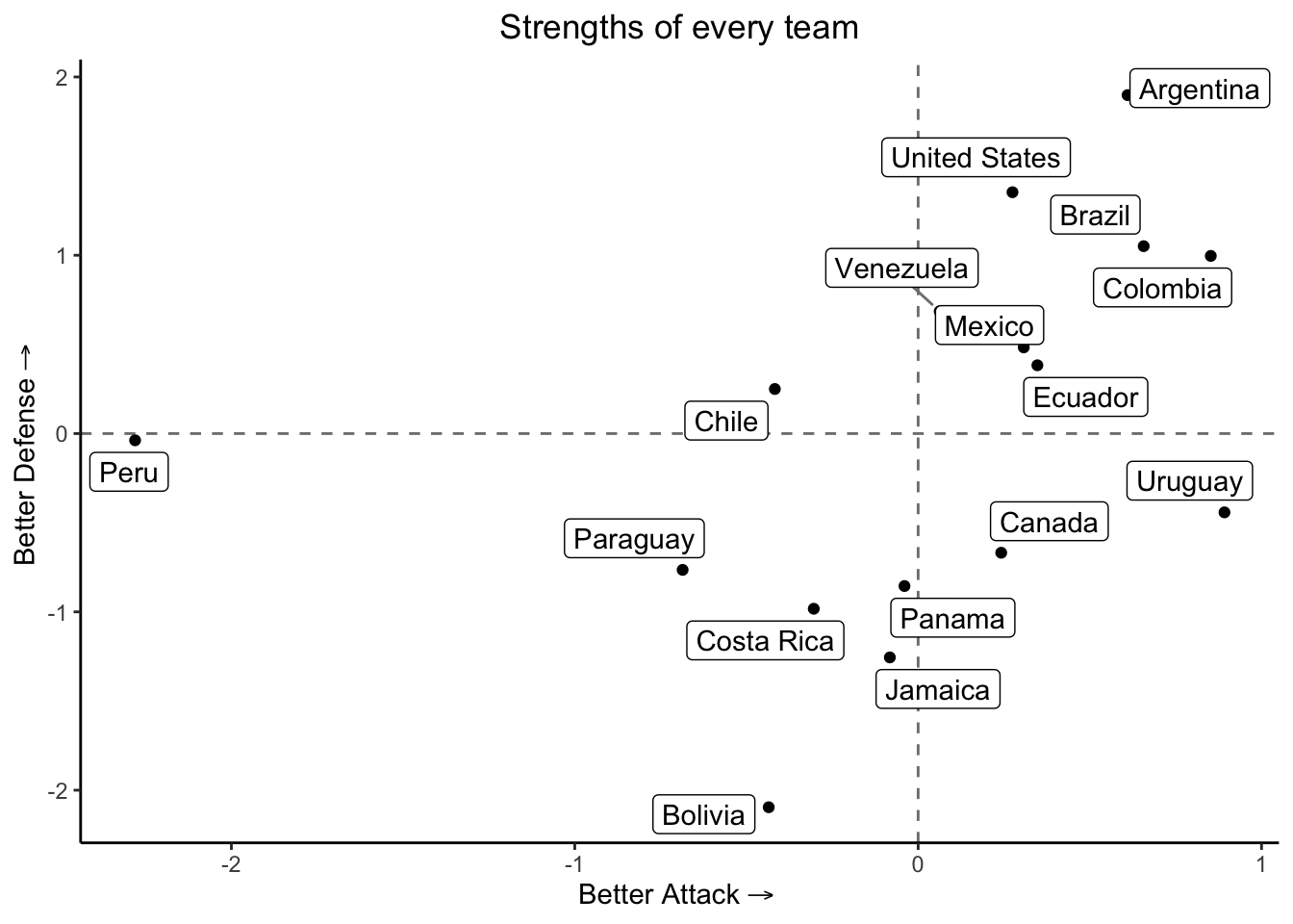
Predictions
Euro
Now, we predict the scores of the future games, i.e, the semifinals and the final.
test_pred <- test_euro %>%
  select(id, team, adversary, condition, ranking_adv)

predictions <- posterior_predict(model_euro, newdata = test_pred)

mean_goals <- apply(predictions, 2, mean)

test_pred <- test_pred %>%
  ungroup() %>%
  mutate(goals = mean_goals) %>%
  group_by(id) %>%
  summarise("Team 1" = first(team),
            "Exp. Goals" = first(goals),
            "Team 2" = last(team),
            "Exp. Goals 2" = last(goals))
The predictions of future games are:
test_pred %>%
  print(n = 1e3)
# A tibble: 101 × 5
id `Team 1` `Exp. Goals` `Team 2` `Exp. Goals 2`
<int> <chr> <dbl> <chr> <dbl>
1 103 France 0.394 Spain 0.831
2 104 England 1.91 Netherlands 1.60
3 105 England 0.620 Spain 1.53
4 106 Croatia 1.55 Portugal 1.29
5 107 Poland 2.15 Scotland 0.938
6 108 Denmark 0.738 Switzerland 0.938
7 109 Serbia 0.350 Spain 1.88
8 110 France 1.27 Italy 0.657
9 111 Austria 1.90 Slovenia 1.33
10 112 Germany 2.16 Hungary 0.875
11 113 Czech Republic 1.84 Georgia 1.86
12 114 Albania 1.42 Ukraine 0.786
13 115 Portugal 2.22 Scotland 0.755
14 116 Croatia 1.94 Poland 1.25
15 117 Denmark 1.05 Serbia 0.487
16 118 Spain 1.28 Switzerland 0.655
17 119 Belgium 0.676 France 0.853
18 120 Germany 2.04 Netherlands 2.00
19 121 Albania 4.49 Georgia 1.19
20 122 Czech Republic 1.06 Ukraine 1.40
21 123 Belgium 1.14 Italy 0.865
22 124 Hungary 1.71 Netherlands 2.44
23 125 Albania 1.91 Czech Republic 0.839
24 126 Georgia 1.08 Ukraine 2.04
25 127 Croatia 3.48 Scotland 0.753
26 128 Poland 1.47 Portugal 1.11
27 129 Serbia 0.522 Switzerland 1.20
28 130 Denmark 0.442 Spain 1.78
29 131 Belgium 0.801 France 0.708
30 132 Germany 2.41 Netherlands 1.67
31 133 Albania 3.92 Georgia 1.43
32 134 Czech Republic 0.678 Ukraine 1.06
33 135 Portugal 2.05 Scotland 0.911
34 136 Croatia 1.65 Poland 1.47
35 137 Serbia 0.310 Spain 2.25
36 138 Denmark 0.625 Switzerland 1.08
37 139 Belgium 1.33 Italy 0.724
38 140 Poland 1.24 Portugal 1.35
39 141 Croatia 2.93 Scotland 0.918
40 142 Denmark 0.507 Spain 1.48
41 143 Serbia 0.438 Switzerland 1.41
42 144 Hungary 1.44 Netherlands 2.89
43 145 Albania 2.24 Czech Republic 0.707
44 146 Georgia 1.68 Ukraine 2.60
45 147 France 1.08 Italy 0.791
46 148 Austria 2.23 Slovenia 1.12
47 149 Croatia 1.84 Portugal 1.09
48 150 Poland 2.70 Scotland 0.788
49 151 Denmark 0.917 Serbia 0.589
50 152 Spain 1.54 Switzerland 0.553
51 153 Germany 1.84 Hungary 1.07
52 154 Albania 2.16 Ukraine 1.05
53 155 Czech Republic 2.25 Georgia 1.54
54 156 Croatia 1.06 France 1.18
55 157 Denmark 1.16 Portugal 0.827
56 158 Germany 1.46 Italy 1.18
57 159 Netherlands 1.08 Spain 2.58
58 160 Austria 2.61 Serbia 0.651
59 161 Hungary 1.29 Turkey 1.77
60 162 Belgium 1.05 Ukraine 0.526
61 163 Slovakia 0.906 Slovenia 1.39
62 164 Albania 1.67 England 2.09
63 165 Croatia 0.896 France 1.39
64 166 Germany 1.69 Italy 0.969
65 167 Denmark 0.995 Portugal 0.997
66 168 Netherlands 0.902 Spain 3.10
67 169 Belgium 1.60 Ukraine 0.668
68 170 Hungary 1.47 Turkey 1.48
69 171 Austria 2.23 Serbia 0.779
70 172 Slovakia 0.764 Slovenia 1.65
71 173 Germany 1.85 Portugal 0.924
72 174 France 0.388 Spain 0.838
73 175 Austria 3.40 Romania 1.53
74 176 Albania 1.85 Serbia 0.621
75 177 France 0.950 Germany 1.02
76 178 Portugal 0.368 Spain 1.51
77 179 Croatia 2.35 Czech Republic 0.807
78 180 Germany 1.94 Slovakia 0.940
79 181 Georgia 1.74 Turkey 2.95
80 182 Netherlands 2.46 Poland 1.60
81 183 Denmark 2.12 Scotland 0.578
82 184 France 0.991 Ukraine 0.466
83 185 Spain 2.32 Turkey 0.666
84 186 Slovenia 0.732 Switzerland 1.16
85 187 Hungary 1.31 Portugal 1.30
86 188 England 1.79 Serbia 0.797
87 189 Croatia 2.00 Czech Republic 0.962
88 190 Georgia 0.529 Spain 5.35
89 191 Albania 1.57 Serbia 0.749
90 192 Austria 2.85 Romania 1.80
91 193 Slovenia 0.876 Switzerland 0.989
92 194 Georgia 1.47 Turkey 3.57
93 195 Hungary 1.09 Portugal 1.56
94 196 France 1.55 Ukraine 0.623
95 197 England 2.11 Serbia 0.659
96 198 Netherlands 2.07 Poland 1.90
97 199 Georgia 0.630 Spain 4.53
98 200 Albania 1.99 England 1.77
99 201 Germany 2.27 Slovakia 0.783
100 202 Denmark 1.81 Scotland 0.694
101 203 Spain 2.70 Turkey 0.558Particullarly, the distribution of the prediction of the score for the final looks as shown below.
results_game <- tibble("England" = predictions[,5], "Spain" = predictions[,6])

df_count <- results_game %>%
  group_by(England, Spain) %>%
  summarise(count = n(), .groups = "keep") %>%
  ungroup()

total_combinations <- nrow(results_game)

df_count <- df_count %>%
    mutate(proportion = count/total_combinations)

ggplot(df_count, aes(x = England, y = Spain, fill = proportion)) +
  geom_tile() +
  scale_fill_gradient(low = "white", high = "blue") +
  labs(title = "Heatmap of Goals Scored by the two teams",
       x = "England",
       y = "Spain",
       fill = "Probability") +
  theme_minimal()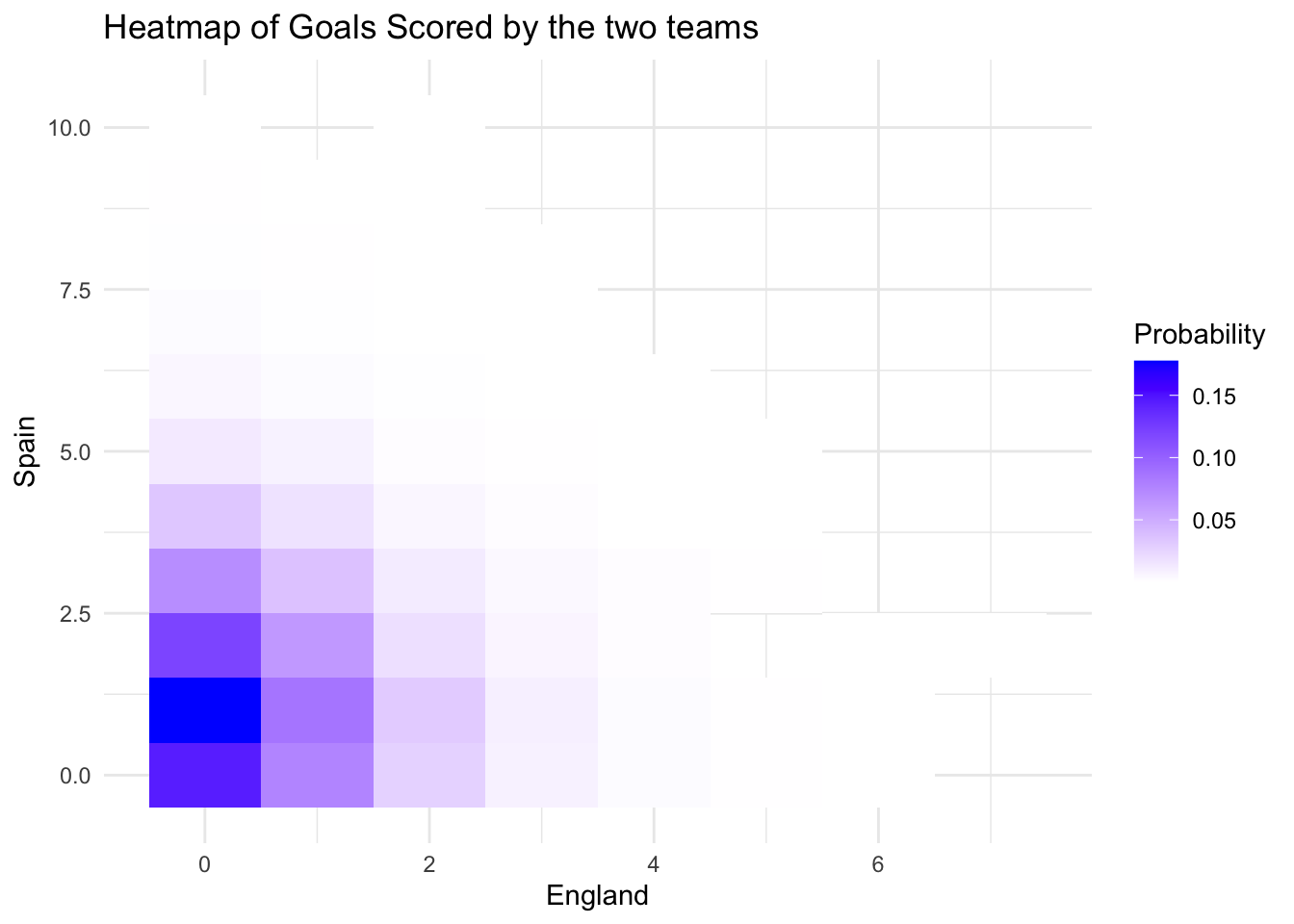
According to this, it is likely that the final will be Spain vs. England. Spain is expected to be the champion, with a predicted score of 2-0.
Copa America
Similarly, we can generate the predictions for the last round of the games in Copa América
test_pred <- test_america %>%
  select(id, team, adversary, condition, ranking_adv)

predictions <- posterior_predict(model_america, newdata = test_pred)

mean_goals <- apply(predictions, 2, mean)

test_pred <- test_pred %>%
  ungroup() %>%
  mutate(goals = mean_goals) %>%
  group_by(id) %>%
  summarise("Team 1" = first(team),
            "Exp. Goals" = first(goals),
            "Team 2" = last(team),
            "Exp. Goals 2" = last(goals))
test_pred %>%
print(n = 1e3)# A tibble: 100 × 5
id `Team 1` `Exp. Goals` `Team 2` `Exp. Goals 2`
<int> <chr> <dbl> <chr> <dbl>
1 96 Argentina 1.91 Canada 0.43
2 97 Colombia 0.868 Uruguay 1.33
3 98 Canada 0.500 Uruguay 2.57
4 99 Argentina 1.01 Colombia 0.752
5 100 Bolivia 0.551 Venezuela 1.64
6 101 Argentina 1.09 Chile 0.180
7 102 Colombia 1.27 Peru 0.108
8 103 Paraguay 0.164 Uruguay 2.35
9 104 Brazil 1.59 Ecuador 0.701
10 105 United States 2.04 United States 2.04
11 106 Canada 1.06 Mexico 1.80
12 107 Argentina 0.882 Colombia 0.942
13 108 Ecuador 1.25 Peru 0.0719
14 109 Bolivia 0.256 Chile 1.14
15 110 Uruguay 1.32 Venezuela 0.747
16 111 Brazil 1.19 Paraguay 0.417
17 112 Bolivia 0.477 Colombia 2.88
18 113 Ecuador 1.56 Paraguay 0.281
19 114 Argentina 0.907 Venezuela 0.614
20 115 Brazil 0.633 Chile 0.545
21 116 Peru 0.0745 Uruguay 1.30
22 117 United States 2.72 United States 2.72
23 118 Canada 2.76 Panama 1.07
24 119 United States 0.830 United States 0.830
25 120 Chile 0.325 Colombia 1.20
26 121 Paraguay 0.386 Venezuela 1.10
27 122 Ecuador 0.456 Uruguay 1.97
28 123 Argentina 3.58 Bolivia 0.167
29 124 Brazil 1.60 Peru 0.0731
30 125 Costa Rica 1.55 Panama 0.999
31 126 United States 1.29 United States 1.29
32 127 Brazil 0.944 Venezuela 1.22
33 128 Bolivia 0.342 Ecuador 2.75
34 129 Argentina 1.30 Paraguay 0.204
35 130 Chile 0.365 Peru 0.0756
36 131 Colombia 0.752 Uruguay 1.78
37 132 Costa Rica 1.02 Panama 1.55
38 133 United States 2.00 United States 2.00
39 134 Bolivia 0.719 Paraguay 0.668
40 135 Colombia 1.92 Ecuador 0.669
41 136 Argentina 1.49 Peru 0.0353
42 137 Chile 0.527 Venezuela 0.502
43 138 Brazil 0.947 Uruguay 1.22
44 139 United States 0.989 United States 0.989
45 140 United States 2.10 United States 2.10
46 141 Chile 1.43 Panama 0.327
47 142 Canada 1.05 Mexico 1.94
48 143 United States 2.71 United States 2.71
49 144 Chile 0.484 Paraguay 0.27
50 145 Bolivia 0.359 Peru 0.276
51 146 Brazil 1.42 Colombia 1.17
52 147 Ecuador 1.04 Venezuela 0.806
53 148 Argentina 0.600 Uruguay 0.986
54 149 United States 2.21 United States 2.21
55 150 Mexico 2.30 Panama 0.751
56 151 Bolivia 0.327 Uruguay 3.03
57 152 Colombia 2.53 Paraguay 0.250
58 153 Peru 0.0671 Venezuela 1.30
59 154 Argentina 1.44 Brazil 0.504
60 155 Chile 0.551 Ecuador 0.478
61 156 Brazil 1.02 Ecuador 1.12
62 157 Paraguay 0.254 Uruguay 1.75
63 158 Argentina 0.615 Chile 0.272
64 159 Colombia 1.96 Peru 0.0644
65 160 Bolivia 0.336 Venezuela 2.99
66 161 Bolivia 0.339 Chile 0.876
67 162 Uruguay 1.81 Venezuela 0.492
68 163 Ecuador 0.784 Peru 0.118
69 164 Argentina 1.36 Colombia 0.604
70 165 Brazil 2.11 Paraguay 0.275
71 166 Costa Rica 0.592 Mexico 1.81
72 167 Jamaica 1.62 Panama 1.26
73 168 United States 2.10 United States 2.10
74 169 United States 1.23 United States 1.23
75 170 Bolivia 0.316 Colombia 4.52
76 171 Argentina 1.40 Venezuela 0.400
77 172 Ecuador 1.03 Paraguay 0.419
78 173 Peru 0.0491 Uruguay 2.05
79 174 Brazil 0.989 Chile 0.352
80 175 Argentina 0.955 Ecuador 0.563
81 176 Paraguay 0.284 Peru 0.157
82 177 Bolivia 0.526 Brazil 2.42
83 178 Colombia 1.12 Venezuela 1.12
84 179 Chile 0.341 Uruguay 0.809
85 180 Argentina 1.17 Venezuela 0.502
86 181 Chile 0.555 Peru 0.05
87 182 United States 1.07 United States 1.07
88 183 Colombia 1.83 Mexico 0.828
89 184 Canada 0.822 Colombia 3.28
90 185 Ecuador 0.907 Mexico 1.12
91 186 Canada 1.09 Ecuador 1.60
92 187 Mexico 0.658 Uruguay 1.50
93 188 United States 1.43 United States 1.43
94 189 Canada 0.826 Venezuela 2.12
95 190 Chile 0.468 Peru 0.055
96 191 Mexico 1.22 Paraguay 0.415
97 192 United States 0.651 United States 0.651
98 193 Bolivia 1.37 Panama 1.20
99 194 Mexico 1.86 Panama 0.949
100 195 Bolivia 0.654 Mexico 1.73 In this case, Argentina is expected to easily defeat Canada, and Uruguay will likely beat Colombia. However, Colombia won its game 1-0, so the final will be Argentina vs. Colombia, while the 3rd and 4th place game will be played between Canada and Uruguay.
The final is anticipated to be a close match, with the most likely result being 0-0, as indicated below. However, Argentina is expected to have a slightly higher probability of scoring more goals than Colombia.
results_game <- tibble("Argentina" = predictions[,7], "Colombia" = predictions[,8])

df_count <- results_game %>%
  group_by(Argentina, Colombia) %>%
  summarise(count = n(), .groups = "keep") %>%
  ungroup()

total_combinations <- nrow(results_game)

df_count <- df_count %>%
    mutate(proportion = count/total_combinations)

ggplot(df_count, aes(x = Argentina, y = Colombia, fill = proportion)) +
  geom_tile() +
  scale_fill_gradient(low = "white", high = "blue") +
  labs(title = "Heatmap of Goals Scored by the two teams",
       x = "Argentina",
       y = "Colombia",
       fill = "Probability") +
  theme_minimal()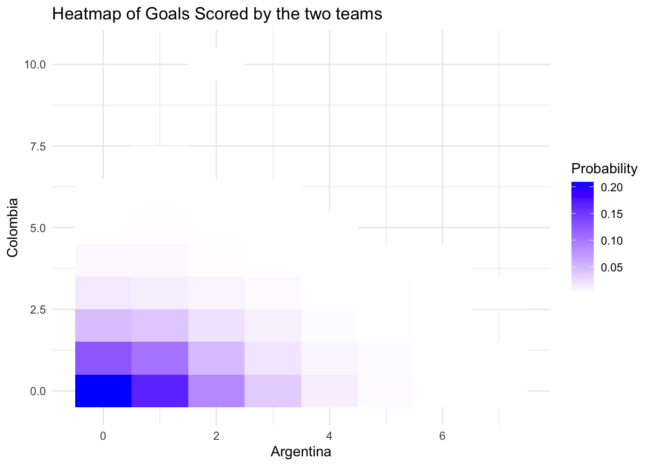
As we saw, the model accurately predicted the scores and captured the strengths of each team. It also produced reasonable and accurate results for the final games based on the quarter-final outcomes. Spain defeated England 2-1, while the match between Argentina and Colombia ended 0-0, with Argentina scoring a goal in extra time.
For future models, incorporating dynamic strengths could improve accuracy.
References
Florez, Mauro, Michele Guindani, and Marina Vannucci. 2024. “Bayesian Bivariate ConwayMaxwellPoisson Regression Model for Correlated Count Data in Sports.” Journal of Quantitative Analysis in Sports 0 (0). https://doi.org/10.1515/jqas-2024-0072.